Suppose that and are both given as functions of a third variable (called parameter ) by the equations

(called parametric equations ). Each value of determines a point ( ), which we can plot in a coordinate plane. As varies, the point ( ) = ( ) varies and traces out a curve C , which is called a parametric curve . If and are defined for all in [ ], then ( f(a), g(a) ) is called the initial point of C and ( f(b), g(b) ) is called the final point of C . Imagine that a particle moving along the curve C , we can interpret as time and ( ) = ( ) as the position of the particle at time . We say C is closed if the initial point and the final point of C are the same.

Consider the curve with parametric equations

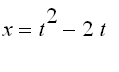
the graphs below show how the curve moves with the parameter .

> with(plots):
  f := t -> t^2 - 2*t:
  g := t -> t + 1:
  c := n -> plot( [ t^2 - 2*t, t + 1, t = -0.001..n ], scaling = constrained,
  thickness = 2 ):
  t := k -> textplot( [ f(k) - 0.34, g(k) + 0.25, `t =` ], 'align = LEFT' ):
  tt := n -> display( seq( t(k), k = 0..n ) ):
  t1 := k -> textplot( [ f(k) - 0.14, g(k) + 0.25, k ] ):
  tt1 := n -> display( seq( t1(k), k = 0..n ) ):
  pp := k -> plot( [ [ f(k), g(k) ] ], style = point, symbol = circle, color = blue ):
  pp1 := n -> display( seq( pp(k), k = 0..n ) ):
  p := n -> display( c(n), tt(n), tt1(n), pp1(n) ):
  display( seq( p(n), n = 0..4 ), insequence = true, scaling = constrained );

Notice that the consecutive points marked on the curve appear at equal time intervals but not at equal distances. That is because the particle slows down and speeds up as increases. Moreover, the curve presented by the parametric equations is part of a parabola .

One of the advantages of parametric description of curves is that they are convenient for "combined motions." This lets us plot curves obtained by adding parametric motions. Here is an example :

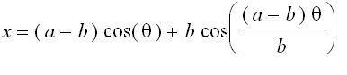
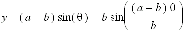
The curve traced out by a point on the circumference of a circle of radius as the circle rolls with a constant angular speed along a straight line is called cycloid . Play the animation below to get a better picture.

A hypocycloid is a curve traced out by a fixed point P  on a circle C  (red) of radius b as C  rolls on the inside of a circle with center O  (blue) and radius a . ( This make more sense physically if a > b , but the curves are just as pretty if a < b .) Play the animation below to get a better picture.

If the initial position of P  is ( ) and the parameter is chosen as in the figure below,

then the parametric equations of the hypocycloid are

The center C  of the smaller circle has coordinates ( ). Since

Arc PS = Arc SQ = ,

thus

so P  has coordinates

.

If circle C  rolls on the outside of the fixed circle O, the curve traced by the point P  is called an epicycloid. Play the animation below to get a better picture.

Similarly, we can show that the parametric equations of the epicycloid are

The center C of the smaller circle has coordinates

( ),

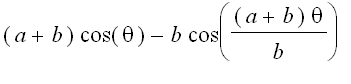
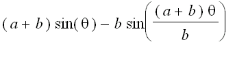
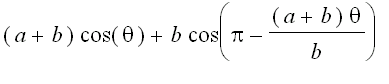
where are radii of the larger circle and the smaller circle, respectively.

Arc PQ has length , so that