ˇ@
Continuity
ˇ@
A function
is continuous at
if
Intuitively speaking,
is continuous at
if
approaches
as
approaches
, as shown in the animation below :
ˇ@
ˇ@
![[Maple Plot]](images_1/suppl_continuity200510/suppl_continuity200510_001.gif)
ˇ@
If
is defined near
, we say
is discontinuous at
(or
has a discontinuity at
), if
is not continuous at
. How can
be discontinuous at
?
ˇ@
Case (i)
exists but
or
is not defined at
,for example
at
.
ˇ@
![[Maple Plot]](images_1/suppl_continuity200527.gif)
In this case, we say
has a removable discontinuity at
, because we can redefine
by
so that
is continuous at
.
ˇ@
Case (ii) Both
and
exist, but
, for example
ˇ@
if
and
if

ˇ@
ˇ@
![[Maple Plot]](images_1/suppl_continuity200541.gif)
In this case,
has a jump discontinuity at
.
ˇ@
Case (iii) Either
or
does not exist, for example
.
ˇ@
ˇ@
ˇ@
![[Maple Plot]](images_1/suppl_continuity200547.gif)
Theorem If
and
are continuous at
and
is a constant, then the following functions are also continuous at
:
1.
2.
3.
4.
if
.
ˇ@
Note that from 1 and 2, we get that
is also continuous at
.
ˇ@
Since
for P , Q polynomials and
, any rational functions is continuous wherever it is defined.
ˇ@
We say
is continuous in an interval, if
is continuous at very number in this interval. Geometrically, we can think of a function that is continuous in an interval as a function whose graph has no break in it. In other words, the graph can be drawn without removing your pen from the paper.
ˇ@
Intermediate Value Theorem
Suppose that
is continuous on the interval
and let
be any number between
and
, where
. Then there exists a number
in (
) such that
.
ˇ@
ˇ@
ˇ@
![[Maple Plot]](images_1/suppl_continuity200573/suppl_continuity200573_001.gif)
ˇ@
The Intermediate Value Theorem says that if
, where
, are in the range of a continuous function
, then the interval
is contained in the range of
.
ˇ@
![[Maple Plot]](images_1/suppl_continuity200579/suppl_continuity200579_001.gif)
ˇ@
We can use the Intermediate Value Theorem to locate roots of equations as in the following example :
Consider the equation
, since
ˇ@
=
and
= 12
ˇ@
The Intermediate Value Theorem says that there is a number
in (
) such that
. In other words, the equation has at least one root in the interval (
). In fact, the Intermediate Value Theorem can help us finding the numerical values of these roots using bisecting algorithm .
ˇ@
The Inverse of a Continuous Function
ˇ@
From the animation below, it is not hard to believe that the inverse of a continuous function is also continuous.
ˇ@
![[Maple Plot]](images_1/suppl_continuity200589.gif)
ˇ@
Suppose that
is strictly increasing and continuous on
. Let
and
and let
be the inverse of
. Note that
is strictly increasing on
. Let
be a number in (
), to show
is continuous at
, we have to show that for each
> 0 there is a
> 0 such that
ˇ@
<
whenever
<
![y[0]+delta](images_1/suppl_continuity2005107.gif)
ˇ@
Let
, so that
. Suppose
is given, without loss of generality, we may assume that
is very small that both
and
are in
.
ˇ@
Let
, see the diagram below .
![[Maple OLE 2.0 Object]](images_1/suppl_continuity2005116.gif)
ˇ@
If
<
then
<
. Since is strictly increasing, we get
ˇ@
=
<
<
=
![g(y[0])+epsilon](images_1/suppl_continuity2005125.gif)
ˇ@
Therefore,
is continuous at
.
For each integer n , since
is continuous and increasing on [
), its inverse function
is also continuous on [
).
ˇ@
ˇ@
Question : Suppose that
is a one-to-one continuous function defined on
, is it true that
is monotonic on
(that is,
is increasing or
is decreasing on
) ?
ˇ@
The Intermediate Value Theorem can help us answer this question. Suppose that
is not monotonic on
, then there exist
in
with
<
<
such that
ˇ@
and
![f(c[3]) < f(c[2])](images_1/suppl_continuity2005147.gif)
or
and
![f(c[2]) < f(c[3])](images_1/suppl_continuity2005149.gif)
ˇ@
Without loss of generality, we may assume
and
. Let
be a number between
and
, the Intermediate Value Theorem says that there exist numbers
with
in (
),
in (
) such that
=
, as shown in the graph below, which contradicts to the fact that
is one-to-one. Hence,
is monotonic on
.
ˇ@
ˇ@
ˇ@
![[Maple Plot]](images_1/suppl_continuity2005165/suppl_continuity2005165_001.gif)
ˇ@
Assume that
and
is continuous at
.
Given
> 0, since
is continuous at
, there exists
> 0 such that
ˇ@
whenever
![abs(y-b) < delta[1]](images_1/suppl_continuity2005174.gif)
ˇ@
Since
, there exists
> 0 such that
whenever
<

ˇ@
![[Maple OLE 2.0 Object]](images_1/suppl_continuity2005180.gif)
ˇ@
Hence, if
<
, we have
and then
. So, we have the following :
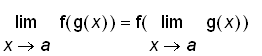
Theorem If
is continuous at
and
, then
. That is,
ˇ@
ˇ@
In other words, the limit symbol can be move through the function symbol.
ˇ@
Consequently, If
is continuous at
and
is continuous at
, then the composition function f o g is continuous at
.
ˇ@
ˇ@
Example Show that the function
is continuous on [
].
ˇ@
Solution :
Since
is continuous on on [
] ,
for all x in on [
] and
is continuous for all
. By the above theorem,
is continuous on [
].
ˇ@
ˇ@
Question : Suppose that
, f is defined at b and
exists, is it true that
ˇ@
?
ˇ@
ˇ@
The following example show that if we replace the continuity condition on f by the existence of
, then the above theorem will not be true even that f is well defined at b .
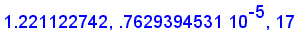
If
and
, then
. We get
ˇ@
and
.
ˇ@
Therefore,
.
ˇ@
ˇ@
ˇ@
