¡@

Double Integrals and Iterated Integrals

Download Maple Worksheet

First let's recall the basic facts about definite integrals of one-variable functions. If  is continuous for all  on [], the definite integral of  on [] is given by the limit of Riemann sums:

where and is any point in  []  for all , ..., .

If  on [],  represents the area of the region bounded by the graph of   , ,  and the  -axis.

 

In a similar manner, we consider a function of two variables continuously defined on a closed rectangle

and we first suppose that . The graph of  is a surface with equation . Let  be the solid that lies above  =  and under the graph of , that is,

What is the the volume of ?

If we take  on  x [], here is the graph of .

Dividing the interval [] into subintervals [] of equal length  and dividing the interval [] into subintervals [] of equal length , We divide the rectangle  into subrectangles

x []

of area , where , .  If we pick a sample point () in each , then we can approximate  by "thin" rectangular columns.

The graph below shows the case where () is taken to be such that  is the minimum value of over :

While the graph below shows the case where () is taken to be such that  is the maximum value of over  :

Notice that the sum of the volume of all these "thin" rectangular columns equals to

 -----  (1)

¡@

Note that the sum in (1) equals

 

As and  go larger, the sum in (1) with to be the maximum value of  over  gets smaller and the sum in (1) with to be the minimum value of  over gets larger, as shown in the animation below :

 

 

So we would expect the they eventually would reach the same value which should be the volume of . In this case, no matter how we choose the sample point (), the sum in (1) would still approach to volume of . The animation below shows the case that () is taken to be  () :

  3DVIEW

So the volume of equals to

 

Definition   The double integral  of   over the rectangle  is

if the limit exists. The sum

 

is called a double Riemann sum .

When  f   is a nonnegative function, the double integral  can be interpreted as the volume of the solid under the surface  and above the region R  in the xy -plane. If f   is not a nonnegative function, the double integral  can be can be interpreted as the "signed volume" (that means we take the volume of the solid above xy-plane to be positive and the volume of the solid under xy-plane to be negative) of the solid between the surface  and in the xy -plane over the region R .

Properties of Double Integrals

1. .

2. , where  is a constant.

3. If  for all ( ) in R, then .

How to compute the double integrals ?

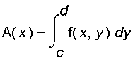
Suppose that  is continuous over  x [] (so for each in [],  is continuous, for all  in [].). For each  in [], we can define

Note that  is continuous on [].

If we now integrate the function with respect to  from to , we get

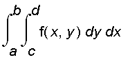
The integral above is called an iterated integral . Usually, the brackets are omitted. Thus,

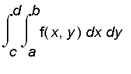
Similarly, the iterated integral

Let and .

Recall that if  is continuous on , the volume of  can be approximate by

.

 

Fixed , , the volume of each thin slice, is approximately equal to

.

So  is approximately equal to

,

as  goes to infinity,  the right hand side of the above equation approaches

.

So we have

 =

Similarly,  the volume of  can be approximate by .

 

For fixed , the volume of each thin slice is approximately equal to

  .

So  is approximately equal to

  ,

a s  goes to infinity, the right hand side of the above equation approaches

So we get

 =

¡@

¡@

Fubini's Theorem

If   f  is continuous on the rectangle x  [], then

=  =

More generally, this is true if we assume that  is bounded on ,   is discontinuous only on a finite number of smooth curves, and the iterated integrals exist.

¡@

¡@

Example:   Evaluate the double integral , where R  = [] x  [].

3DVIEW

Note that the surface  lies below the xy -plane, so the double integral should be negative.

¡@

Solution : Fubini's theorem gives

 =  =  

¡@

Example:  Evaluate the double integral , where R  = [] x  [].

3DVIEW

Solution : We integrate with respect to x first,

=  = 0

¡@

Remarks :

1. If we integrate with respect to y  first, the computation will be much more complicated.

2. = 0 says that the volume of the solid under the surface , above the xy-plane over  equals to of the solid above the surface , below the xy-plane over  are equal.  

3DVIEW

Example:  Find the volume of the solid S that is bounded by , the planes  and , and the three coordinate planes.

3DVIEW

Solution : Note that is  positive on [ ] x  [ ], so the volume equals to

 =

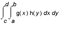
Note that in the special case where  and x [], the Fubini's theorem gives

  =     

                         =  

                        =  

                           =  

---

Download Maple Worksheet