ˇ@
Partial Derivatives
Consider a two variable function
, suppose we let only
vary while keeping
fixed, say
, where
is a constant. Then we are really considering a function of a single variable
, namely
. If
has a derivative at
, then we call it the partial derivative of
with respect to
at (
,
) and denote it by
(or
).
Thus by the definition of a derivative we have:

Similarly, the partial derivative of
with respect to
at (
,
),
(or
) is given by:

Let's consider the function
, the graphs below show the geometric meaning of
and
:
Here is an alternate geometric interpretation for the partial derivative in terms of vector functions:
Let
and the graph
of the function
(viewed on the plane
.) is the curve traced out by the vector function G (
)=(
) whose vector derivative G '(
)=(
) is determined by
. (That is, its "slope" is
.)
similarly, the graph of
is the curve
traced out by the vector function H (
)=(
) whose vector derivative H '(
)=(
) is determined by
.
Now let's take a look at a function
which is not continuous at (
,
), but
exists at (
). Let
for all (
,
) except at (
,
), and
.
As we can see from the graphs above,
along
,
and
for all (
) except at (
) along
. So that
is not continuous at (
,
) (
does not exist), but
,
if (
) = (
).
ˇ@
Note that
and
for all (
) other than (
,
).
ˇ@
ˇ@
Now let's consider the partial derivatives of the function
.
and
.
,
,
,
and
.
Here are the graphs of the partial derivatives :
Notice that here we have
, but this is not true in general.
Let's go back to the function
for all (
,
) except at (
,
), and
.
Since
and
.
ˇ@
We have seen that
,
if (
) = (
) and
and
for all (
) other than (
,
). We get
and
.
In fact, we can also compute them directly from the definition :
.
and
.
It is not hard to see that
and
do not exist at (
,
).
Let's take a look at the function
for all (
,
) except at (
,
),and
.
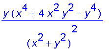
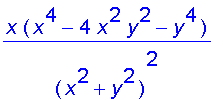
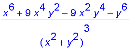
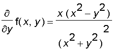
Calculations, which we leave as an exercise, show that
and
.
ˇ@
> diff((x^3*y-x*y^3)/(x^2+y^2),x):
simplify(%);
diff((x^3*y-x*y^3)/(x^2+y^2),y):
simplify(%);


Here are the graphs of
and
.
> x:='x':
y:='y':
diff(diff((x^3*y-x*y^3)/(x^2+y^2),y),x):
simplify(%);
diff(diff((x^3*y-x*y^3)/(x^2+y^2),x),y):
simplify(%);


Here are the graphs of
and
.
Note that
and
are not continuous at (
,
).
Clairaut's Theorem
Suppose that f is defined on a disk D that contains (
). If the functions
and
are continuous on D , then
.
![[Maple Plot]](images/suppl_PartialDerivative27.gif)
![[Maple Plot]](images/suppl_PartialDerivative28.gif)
![[Maple Plot]](images/suppl_PartialDerivative39.gif)
![[Maple Plot]](images/suppl_PartialDerivative47.gif)
![[Maple Plot]](images/suppl_PartialDerivative59.gif)
![[Maple Plot]](images/suppl_PartialDerivative60.gif)
![[Maple Plot]](images/suppl_PartialDerivative84.gif)
![[Maple Plot]](images/suppl_PartialDerivative85.gif)
![[Maple Plot]](images/suppl_PartialDerivative90.gif)
![[Maple Plot]](images/suppl_PartialDerivative91.gif)
![[Maple Plot]](images/suppl_PartialDerivative104.gif)
![[Maple Plot]](images/suppl_PartialDerivative105.gif)
![[Maple Plot]](images/suppl_PartialDerivative106.gif)

![[Maple Plot]](images/suppl_PartialDerivative139.gif)
![[Maple Plot]](images/suppl_PartialDerivative146.gif)
![[Maple Plot]](images/suppl_PartialDerivative147.gif)
![[Maple Plot]](images/suppl_PartialDerivative152.gif)
![[Maple Plot]](images/suppl_PartialDerivative153.gif)